
- Introduction
Remote sensing indicators play a pivotal role in identifying and assessing agricultural droughts due to their unique ability to provide comprehensive and timely information over large geographical areas (Der Sarkissian et al. 2019). These indicators, derived from satellite imagery and sensor data, offer a bird’s-eye view of vegetation health, moisture content, and temperature variations crucial for gauging agricultural conditions. They enable a deeper understanding of vegetation dynamics, allowing for the early detection of stress in crops and vegetation cover. By capturing essential parameters remote sensing indicators facilitate the monitoring of changes in vegetation vigor and response to moisture stress or temperature fluctuations. Their capacity to provide historical, current, and predictive data aids in decision-making processes, guiding agricultural planning, resource allocation, and mitigation strategies to combat the impacts of droughts on crop yield and food security (Al Sayah et al. 2021). Consequently, these indicators contribute significantly to proactive drought management and resilience-building in agricultural systems.
On the other hand, climatic models play a pivotal role in understanding and predicting the potential impacts of climate change on agriculture, hence providing valuable insights that are crucial for sustainable food production. For agriculture, these predictions are indispensable for anticipating shifts in growing seasons, identifying regions at risk of extreme weather events, and assessing changes in water availability. Farmers, policymakers, and researchers can use this information to develop adaptive strategies, optimize crop selection, and implement resilient farming practices. With their capacity to give insights from the future, corresponding decision making, and implementation of proactive and reactive measures equally is ensured.
In this context, the following study gives a brief example on the capacity of remote sensing indicators and climatic geospatial data for monitoring vegetation health and climatic conditions of heatwaves in St Emilion for the summer of 2023.
2. Methodology
2.1. Remote sensing indicators
The Vegetation Health Index (VHI) combines the Vegetation Condition Index (VCI) and the Temperature Condition Index (TCI) to evaluate both vegetation and temperature stress. VHI is a valuable tool for detecting drought (Kogan 1995) and is particularly noted for its effectiveness in assessing extensive areas (Yan et al. 2016).
The formula for computing VHI is as follows (Eq 1):

Different VHI values correspond to various drought classifications as defined by Kogan (1995): > 40 (no drought), 30–40 (mild drought), 20–30 (moderate drought), 10–20 (severe drought), and < 10 (extreme drought).
To calculate VHI, one must initially compute the VCI and TCI indices. VCI quantifies vegetation dynamics on a scale of 0–100 to reflect moisture changes (Bhuiyan, 2008) using this equation (Eq 2):
The NDVI (Normalized Difference Vegetation Index) calculation is derived from Red and NIR bands, indicating vegetation presence based on spectral reflectance (intensity of red color) (Eq 3):
NDVI ranges from − 1 to 1, higher values signifying healthy vegetation and lower values suggesting sparse vegetation (Singh et al. 2016). The extraction of NDVI was accomplished using the “Raster Calculator” tool in ArcGIS (ESRI 2016) through specific equations based on different LANDSAT platforms.
LANDSAT 4, 5, and 7: NDVI = Float ((“Band 4” – “Band 3”))/Float ((“Band 4” – “Band 3”))
LANDSAT 8: NDVI = Float ((“Band 5” – “Band 4”))/ Float ((“Band 5” + “Band 4”))
Once the NDVI rasters were obtained, VCI was calculated for various years using Eq. 2. TCI, on the other hand, represents Temperature Condition Index, capturing vegetation responses to temperature shifts. TCI complements VCI in offering more accurate drought assessments (Sholihah et al. 2016) and is computed using this formula (Eq 4):
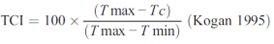
where Tc, Tmin, and Tmax are values corresponding to Land Surface Temperatures (LST). TCI values range from 0 to 100, lower values indicating vegetation stress due to temperature or drought elevations (Bhuiyan 2008). TCI’s advantage lies in its applicability throughout any season, unlike VCI, since it relies on Land Surface Temperatures (LST) (Yan et al. 2016). LST, extracted from thermal bands of satellite platforms, particularly LANDSAT, is a crucial element for TCI computation. The thermal sensor of LANDSAT platforms measures top-of-atmosphere radiances, allowing for brightness temperature extraction using Plank’s law (Dash et al. 2002). The steps for LST extraction are outlined in Table 1 according to the LANDSAT user data guide handbook.
Table 1. Calculation of LST from LANDSAT images
| Steps | Equations from Avdan and Jovanovska |
| 1 – Conversion of Digital Number (DN) to radiance | 𝑳λ=((𝐋𝐌𝐀𝐗𝛌−𝐋𝐌𝐈𝐍𝛌)(𝐐𝐂𝐀𝐋𝐌𝐀𝐗− 𝐐𝐂𝐀𝐋𝐌𝐈𝐍))∗(𝐐𝐂𝐀𝐋−𝐐𝐂𝐀𝐋𝐌𝐈𝐍)+𝐋𝐦𝐢𝐧𝛌 |
| 2- Conversion of radiance into satellite temperature | 𝑻= 𝐾2𝐿𝑛(𝐾1𝐿𝛌+1) – 273.15 |
| 3- Calculation of the proportion of vegetation (Pv) | 𝑷𝒗= [(𝑁𝐷𝑉𝐼−𝑁𝐷𝑉𝐼𝑚𝑖𝑛)(𝑁𝐷𝑉𝐼max− 𝑁𝐷𝑉𝐼 min )]2 |
| 4- Calculation of the surface emissivity (LSE) | LSE = 0.004 * Pv + 0.986 |
| 5- Extraction of LST | 𝑳𝑺𝑻= 𝑇1+λ∗(𝑇𝑝)∗𝐿𝑛(𝐿𝑆𝐸) |
With Lλ the spectral radiation at the sensor aperture in (watts/m2*ster*μm), QCAL is the quantized calibrated pixel value in DN, LMINλ is the spectral radiation which is scaled to QCALMIN (in watts /m2* ster* μm) , LMAXλ is the spectral radiance which is scaled for QCALMAX (in watts/ m2* ster* μm), QCALMIN is the quantized minimum calibrated pixel value (corresponding to LMINλ) in DN, QCALMAX is the quantized maximum calibrated pixel value (corresponding to LMAXλ ) in DN, T is the effective temperature of the satellite in Kelvin (we added -273.15 as a conversion factor from Kelvin to ˚C), K1 is the constant of band-specific thermal conversion (in watts/m2 * ster * μm), K2 is the thermal band-specific thermal conversion constant (in Kelvin), λ is the wavelength of the emitted radiation, ρ is the h * c / σ (1.438 × 10⁻² m ∙ K), h is Planck’s constant (6.626 × 10⁻³⁴ J ∙ s), σ is Boltzmann’s constant (1.38 × 1 0−23 J/K) and c is the speed of light (2.998 × 10⁸ m/s).
After obtaining the LST index for the entire studied period, TCI was calculated using the “Raster Calculator” tool as specified. Finally, with VCI and TCI maps in hand, VHI computation followed.
2.2. Climatic indicator
In the case of St Emilion, frost and icing conditions are becoming major preoccupations. Understanding the evolution of these phenomena is key for anticipatory planning. Accordingly, MeteoFrance’s DRIAS database was used to obtain the “Number of Frost Days” indicator defined as: The number of days for which the daily minimum temperature of day i is less than or equal to 0. The temporal reference was selected for the reference period (1976-2005) and the year 2050.
Data was obtained in shapefile format, then rasterized to be downscaled to 1 km. By transposing the layer points, the gridded layer will be assimilated to a weather station network. Since the different points holding different climatic values can be considered as “spatial weather stations”. Through a specific kriging technique, spatiotemporal variations were calculated. As most data is transposed into GIS format, a detailed spatiotemporal evolution is obtained. Accordingly, areas of vulnerability are highlighted, hence allowing subsequent prioritized proactive and/or reactive measures. That way, evidence and priority-based budget allocation for orienting interventions can be offered. The reference period and the RCP8.5 scenario were chosen for this example. RCP8.5, the pessimistic climatic pathway was chosen to present the most plausible extreme conditions. By subtracting the predicted horizon and the reference period findings, anomalies were obtained.
3. Results and discussions
3.1. Remote sensing indicators
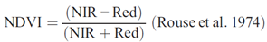
In this section, the findings of the remote sensing indicators will be detailed. NDVI, TCI, VCI and VHI will be discussed with respect to the obtained values and geographical gradients on the territory.
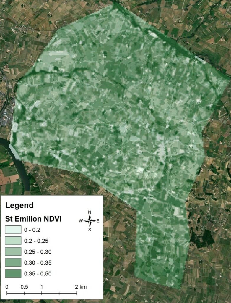
The NDVI map reveals the presence of healthy and dense vegetation with increasing values. As can be seen, most of Saint Emilion displays high to very high values, hence indicating healthy vegetation. Linear strips can be observed as these correspond to mulches that are often laid between vineyards by farmers as part of vegetative measures.
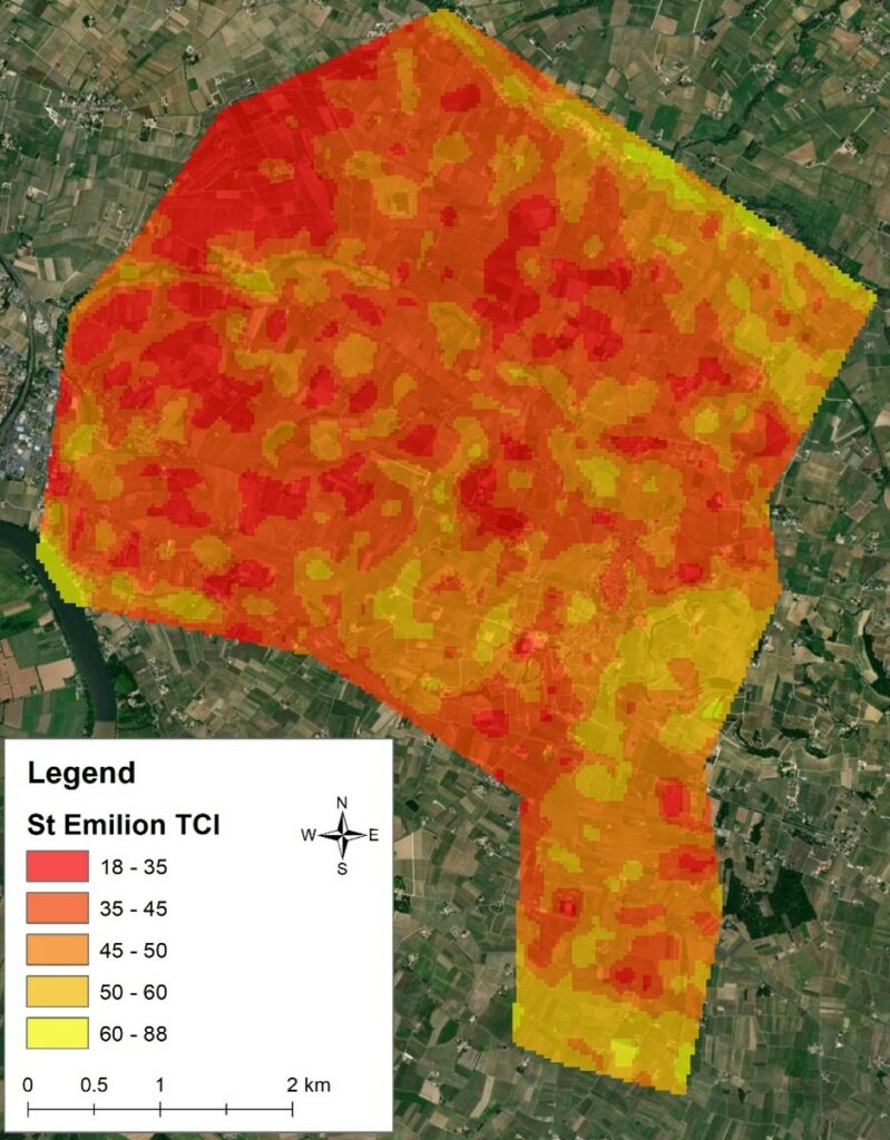
TCI ranges from 0 to 100 with low values indicating vegetation stress due to temperature/drought increases. As can be seen, most of the territory was under thermal vegetation stress particularly in the central and peripheral regions with heat pockets apparent in the Central-Western parts.
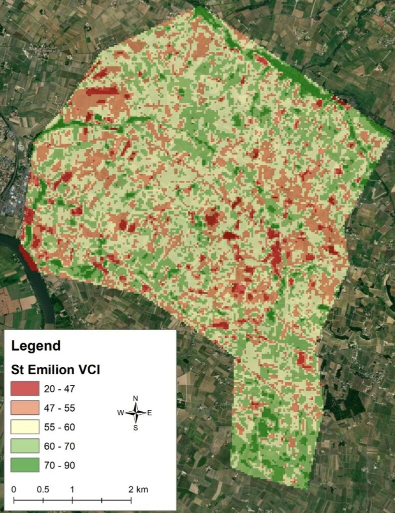
High values of VCI indicate rather a suitable condition of vegetation while lower values indicate stress. As can be seen most of the territory falls under suitable conditions except for parcels located in the North-Central region that display stress.
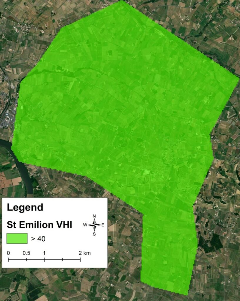
As can be seen from Figure 4, the vegetation health index of St Emilion showed no drought class in terms of VHI.
3.2. Climatic indicator: Evolution of heatwaves
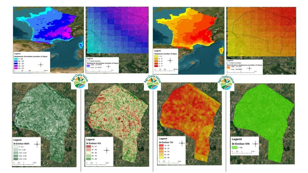
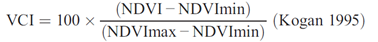
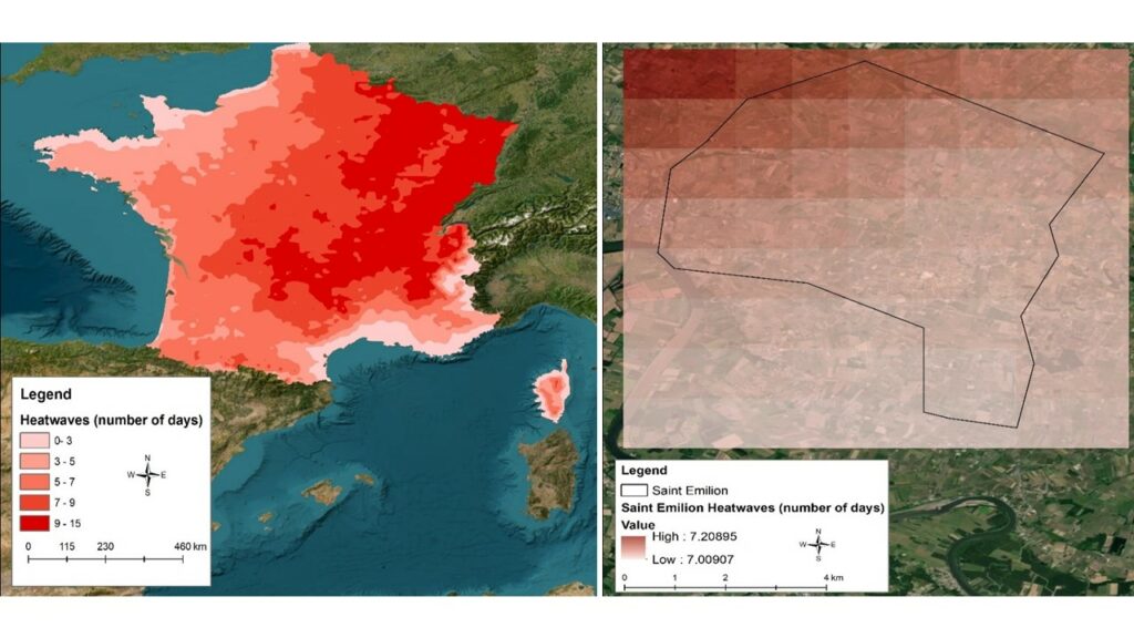
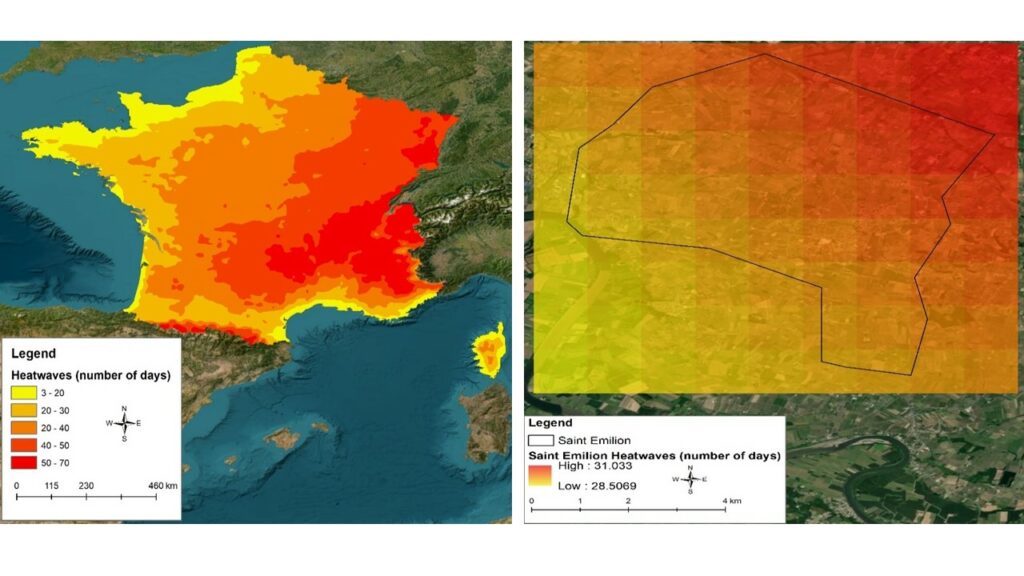
The number of days for heatwaves is revealed in the following maps (Figures 5, 6 and 7). From Figure 5, one can see that the number of heatwaves ranged between 0 and 15 days with the Western region particularly affected. For St Emilion, the number of heatwaves is around 7 days. The highest risks are mainly concentrated in the Northern and Eastern parts of St Emilion and decreases with the progression South and West. In Figure 6, findings show that the number of frost days will significantly increase at the national scale. For St Emilion, number of frost days in 2050 under RCP8.5 are expected to significantly increase from 28 minimum and 31 days maximum (from 7 days) with the same geographical gradient.
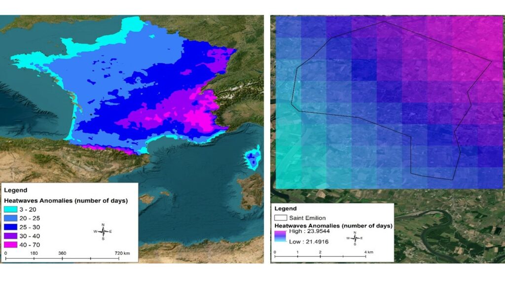
In term of anomalies, generally, a significant increasing trend is observed in throughout the national territory. The same is applicable for St Emilion under the same geographical gradient.
4. Conclusion
In conclusion, the utilization of remote sensing in conjunction with climate indicators emerges as an indispensable approach in the assessment of agricultural drought, revolutionizing the methodology employed in comprehending, monitoring, and responding to environmental adversities. Through the application of remote sensing technologies, access to expansive geographical regions is facilitated, enabling the acquisition of real-time data crucial for informed decision-making in agriculture. This amalgamation not only allows for the early detection and precise monitoring of drought conditions but also facilitates the implementation of proactive measures to alleviate its impact on crops and livelihoods. The deployment of these technologies equips policymakers, farmers, and stakeholders with a robust framework for sustainable agricultural practices, ensuring resilience amidst the evolving patterns of climate change. As society navigates the intricate dynamics of a shifting climate, the fusion of remote sensing and climate indicators assumes a pivotal role, fostering adaptive strategies and fortifying food security for future generations.
References
Al Sayah, M.J., Abdallah, C., Khouri, M., Nedjai, R., Darwich, T., 2021. A framework for climate change assessment in Mediterranean data-sparse watersheds using remote sensing and ARIMA modeling. Theoretical and Applied Climatology. 143, 639–658. https://doi.org/10.1007/s00704-020-03442-7
Der Sarkissian, R., Zaninetti, J.M, Abdallah., C., 2019. The use of geospatial information as support for Disaster Risk Reduction; contextualization to Baalbek-Hermel Governorate/Lebanon, Applied Geography. 111, 102075. https://doi.org/10.1016/j.apgeog.2019.102075
Kogan, FN. 1995. Application of vegetation index and brightness temperature for drought detection. Adv Sp Res 15:91–100
Yan N, Bingfang W, Boken VK, Chang S, Yang L. 2016. A drought monitoring operational system for China using satellite data: design and evaluation. Geomatics Nat Hazards Risk 7:264–277
Bhuiyan C (2008) Desert vegetation during droughts: response and sensitivity. Int Arch Photogramm Remote Sens Spat Inf Sci, XXXVII
Singh RP, Singh N, Singh S, Mukherjee S. 2016 Normalized difference vegetation index (NDVI) based classification to assess the change in land use/land cover (LULC) in Lower Assam, India. Int J AdvRemote Sens GIS 5:1963–1970
ESRI (2016) Raster Calculator [WWW Document]. Spat. Anal. Tools URL https://desktop.arcgis.com/en/arcmap/10.3/tools/spatialanalyst-toolbox/raster-calculator.htm
Sholihah RI, Trisasongko BH, Shiddiq D, Iman LOS, Kusdaryanto S, Manijo PDR. 2016. Identification of agricultural drought extent based on vegetation health indices of Landsat data: case of Subang and Karawang, Indonesia, in: The 2nd International Symposium on LAPAN-IPB Satellite for Food Security and Environmental Monitoring 2015, LISAT-FSEM 2015. In: Procedia Environmental Sciences, pp 14–20. https://doi.org/10.1016/j.proenv.2016.03.051
Dash P, Göttsche FM, Olesen FS, Fischer H. 2002. Land surface temperature and emissivity estimation from passive sensor data: theory and practice-current trends. Int J Remote Sens 23:2563–2594